Want to know how to calculate flux from a halbach array?
You’re in the right place.
These magnetic powerhouses are everywhere in 2025. From maglev trains to MRI machines, they’re revolutionizing how we think about magnetic fields.
But here’s the thing: calculating their flux isn’t exactly straightforward.
In this guide, as a professional Halbach array manufacturer, I’ll walk you through everything you need to know about flux calculations for Halbach arrays. No PhD required.
Sound good? Let’s dive in.
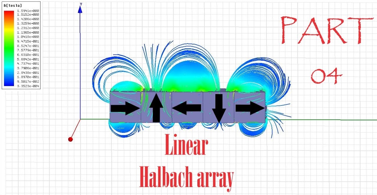
Table of Contents
What is a Halbach Array (And Why Should You Care)?
Picture this: You have a bunch of permanent magnets arranged in a clever pattern. Each magnet rotates 90 degrees from the next one.
The result? Magic.
Well, not really magic. But close.
A Halbach array creates a super-strong magnetic field on one side while practically canceling it out on the other. It’s like having a one-sided magnet (which doesn’t actually exist, but you get the idea).
Here’s why this matters:
- Stronger fields: Up to twice the strength of regular magnet arrangements
- Focused power: All the magnetic energy goes where you want it
- Efficiency: Less wasted magnetic field means better performance
Bottom line? These arrays are game-changers for any application that needs focused magnetic fields.
The Flux Calculation Challenge
Now, here’s where things get tricky.
Unlike regular magnets, Halbach arrays don’t have simple, straightforward formulas for flux calculation. The magnetic field varies dramatically depending on:
- Array geometry (linear, cylindrical, spherical)
- Distance from the array
- Number of magnet segments
- Individual magnet properties
But don’t worry. I’m going to break this down into manageable chunks.
Understanding Magnetic Flux (The Basics)
Before we jump into the nitty-gritty, let’s make sure we’re on the same page about flux.
Magnetic flux is basically the amount of magnetic field passing through a specific area. Think of it like counting how many magnetic field lines cross an imaginary surface.
The formula is dead simple:
Φ = B × A
Where:
- Φ (phi) = magnetic flux (measured in Webers)
- B = magnetic field strength (measured in Tesla)
- A = area (measured in square meters)
Easy enough, right?
The challenge with Halbach arrays is that B (magnetic field strength) isn’t constant. It varies based on position, distance, and array configuration.
That’s what makes the calculation more complex.
Types of Halbach Arrays (And Their Flux Characteristics)
Not all Halbach arrays are created equal. Each type has different flux calculation methods.
Linear Halbach Arrays
These are the flat, straight-line arrangements you see most often.
The magnetic field on the “strong” side follows this pattern:
B(z) = Br × (1 – e^(-kz))
Where:
- Br = remanence of the magnetic material
- k = wave number (k = 2π/L, where L is the period)
- z = distance from the array surface
The field decays exponentially as you move away from the array. This is crucial for flux calculations.
Cylindrical Halbach Arrays
Think electric motors and generators.
For cylindrical arrays, the flux density inside the bore is:
B_bore = (M0/μ0) × ln(Ro/Ri)
Where:
- M0 = magnet remanence
- μ0 = vacuum permeability
- Ro = outer radius
- Ri = inner radius
Pro Tip: The logarithmic relationship means small changes in radius ratios can significantly impact flux density.
Spherical Halbach Arrays
These are the exotic ones. Mostly used in specialized research applications.
The field inside a spherical array is:
B = (4/3) × M0 × ln(Ro/Ri)
Notice the 4/3 factor? That’s what gives spherical arrays their unique characteristics.
Step-by-Step Flux Calculation Methods
Alright, let’s get practical. Here are the three main approaches you can use.
Method 1: Analytical Approach (For Simple Cases)
This works best for basic geometries and uniform fields.
Step 1: Define your parameters
- Array type and dimensions
- Magnet material properties (Br, μr)
- Measurement area and distance
Step 2: Calculate field strength
Use the appropriate formula from the previous section.
Step 3: Integrate over the area
For uniform fields: Φ = B × A
For varying fields: Φ = ∫∫ B·dA
Let me show you a real example:
Cylindrical Array Calculation:
- M0 = 1.3 T (neodymium magnet)
- Ro = 0.1 m, Ri = 0.05 m
- Calculate flux through bore cross-section
B_bore = (1.3 T)/(4π × 10^-7) × ln(0.1/0.05)
B_bore ≈ 0.72 T
Φ = 0.72 T × π × (0.05 m)²
Φ ≈ 0.0057 Wb
That’s your total flux through the area.
Method 2: Numerical Integration (For Complex Geometries)
When analytical solutions don’t cut it, numerical methods save the day.
The process:
- Discretize the surface into small elements
- Calculate B at each element center
- Sum up contributions: Φ = Σ(Bi × ΔAi)
This approach handles:
- Non-uniform fields
- Irregular surfaces
- Complex array geometries
- Edge effects
Method 3: Finite Element Analysis (FEA)
For serious engineering work, FEA is your best friend.
Software options:
- COMSOL Multiphysics (industry standard)
- ANSYS Maxwell (electromagnetic specialist)
- FEMM (free alternative)
These tools model the complete magnetic field distribution and calculate flux through any defined surface.
The advantage? They account for real-world factors like:
- Finite magnet sizes
- Material non-linearities
- Temperature effects
- Manufacturing tolerances
Real-World Adjustments (Making Theory Meet Reality)
Here’s where theory meets the messy real world.
Perfect formulas assume perfect conditions. But real Halbach arrays have imperfections that affect flux calculations.
Magnet Permeability Correction
Permanent magnets aren’t perfectly linear. For neodymium magnets (μr ≈ 1.05), multiply your calculated B field by:
Correction factor = 1/√μr ≈ 0.976
Small change, but it matters for precision applications.
Segmentation Effects
Using discrete magnet pieces instead of continuous magnetization? Apply this correction:
Correction = sin((k+1)π/N) / ((k+1)π/N)
Where N = number of segments.
More segments = closer to ideal performance.
Finite Size Effects
Short arrays don’t behave like infinite ones. For cylindrical arrays with length L and radius R:
If L/R < 5, expect significant field reduction at the ends.
Temperature Dependencies
Magnetic properties change with temperature. For NdFeB magnets:
Br(T) = Br(20°C) × [1 – α(T – 20°C)]
Where α ≈ 0.0012/°C for typical neodymium magnets.
In hot environments, this can significantly impact your flux calculations.
Practical Measurement and Validation
Calculations are great. But measurement validates everything.
Using Gaussmeters
A calibrated gaussmeter measures B directly. Take readings at multiple points and integrate numerically:
Φ ≈ Σ(Bi × Ai)
Search Coil Method
Wind a precise coil around your measurement area. Extract it rapidly and measure the induced EMF:
Φ = ∫(EMF dt) / Nturns
This gives you the total flux through the coil area.
Hall Sensor Arrays
Multiple Hall sensors create a field map. Interpolate between measurement points and integrate over your surface.
Pro Tip: Always validate calculations against measurements. Theory and practice sometimes disagree.
Common Mistakes (And How to Avoid Them)
After working with magnetic field calculations for years, I’ve seen these errors repeatedly:
Mistake #1: Ignoring Edge Effects
The Problem: Using infinite array formulas for finite arrays.
The Fix: Add at least one wavelength of “buffer” magnets beyond your measurement area.
Mistake #2: Wrong Coordinate Systems
The Problem: Mixing up radial, axial, and angular components.
The Fix: Draw clear diagrams showing your coordinate system before calculating.
Mistake #3: Temperature Neglect
The Problem: Using room temperature properties for all conditions.
The Fix: Always apply temperature corrections for your operating environment.
Mistake #4: Linear Superposition Assumptions
The Problem: Adding fields algebraically instead of vectorially.
The Fix: Remember that magnetic fields are vectors. Direction matters.
Advanced Optimization Techniques
Want to maximize flux for your application? Here are some pro strategies:
Magnet Grade Selection
Higher grade magnets = stronger fields. But they’re also more expensive and temperature-sensitive.
N52 grade: Maximum strength, limited temperature range
N42 grade: Good balance of performance and stability
N35 grade: Lower cost, wider temperature range
Array Geometry Optimization
The optimal geometry depends on your flux requirements:
- Maximize peak field: Use cylindrical arrays with high Ro/Ri ratios
- Maximize uniformity: Use longer arrays with gradual field transitions
- Minimize cost: Use fewer, larger magnets (but accept some performance loss)
Multi-Layer Designs
Stack multiple Halbach layers for enhanced performance:
Btotal = Σ(Bk × e^(-kk×z))
Each layer contributes according to its position and spacing.
Applications and Industry Examples
Let’s talk real-world applications where accurate flux calculations matter:
Electric Motors
High-performance motors use Halbach rotors for maximum torque density. Flux linkage calculations determine:
- Motor constant (Kt)
- Back EMF characteristics
- Efficiency predictions
Magnetic Levitation
Maglev systems require precise flux calculations for:
- Lifting force predictions
- Stability analysis
- Power consumption estimates
MRI Systems
Portable MRI machines increasingly use Halbach arrays. Critical calculations include:
- Field homogeneity over imaging volume
- Gradient field interactions
- Patient safety assessments
Particle Accelerators
Wiggler magnets in synchrotrons use specialized Halbach configurations. Engineers calculate:
- Beam deflection angles
- Radiation spectrum characteristics
- Magnetic field quality requirements
Software Tools and Resources
Here are my recommended tools for flux calculations:
Free Options
- FEMM: Excellent for 2D magnetostatic problems
- Agros2D: User-friendly finite element solver
- MATLAB/Octave: Custom calculation scripts
Commercial Software
- COMSOL: Industry standard for multiphysics
- ANSYS Maxwell: Specialized electromagnetic solver
- Opera: High-end 3D electromagnetic analysis
Online Calculators
Several websites offer basic Halbach array calculators. They’re good for quick estimates but limited for serious design work.
Future Developments
The field is evolving rapidly in 2025:
Advanced Materials
- Rare-earth-free magnets: Reducing dependence on critical materials
- Nanostructured magnets: Enhanced properties through material engineering
- High-temperature magnets: Extending operating ranges
Smart Manufacturing
- Variable magnetization: Creating complex field patterns
- 3D printing integration: Embedding magnets during printing
- AI-optimized designs: Using machine learning for geometry optimization
Hybrid Systems
Combining permanent magnets with electromagnets for adjustable field strength. This adds complexity but enables real-time flux control.
Troubleshooting Common Calculation Issues
When your calculations don’t match measurements, check these common culprits:
Field Measurement Errors
- Probe positioning: Small position errors cause large field variations near arrays
- Temperature drift: Both magnets and sensors change with temperature
- External fields: Earth’s field and nearby ferromagnetic objects
Calculation Assumptions
- Material properties: Manufacturer specs vs. actual performance
- Geometric tolerances: Manufacturing variations affect field distribution
- Assembly gaps: Small air gaps dramatically reduce field coupling
Software Limitations
- Mesh density: Too coarse = inaccurate results
- Boundary conditions: Improper setup skews results
- Convergence criteria: Stopping too early gives wrong answers
Conclusion
How to calculate flux from a halbach array boils down to understanding your specific configuration and choosing the right calculation method.
For simple geometries, analytical formulas work great. For complex real-world applications, numerical methods or FEA provide the accuracy you need.
The key takeaways?
- Start with the basics: Understand your array type and measurement requirements
- Choose appropriate methods: Match calculation complexity to your accuracy needs
- Account for real-world effects: Temperature, tolerances, and finite sizes matter
- Validate with measurements: Theory and practice should agree
Whether you’re designing the next breakthrough motor or optimizing a magnetic separator, these flux calculation principles will serve you well.
The bottom line? Mastering flux calculations opens up a world of magnetic design possibilities. And in 2025, with advancing materials and manufacturing techniques, the potential applications are virtually limitless.
Ready to put this knowledge to work? Start with a simple calculation using the methods I’ve outlined. You’ll be surprised how quickly you can go from theory to practical results.